
PAGE LAYOUT-PRINT AREA
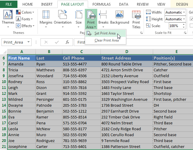
If you prefer, you can also set the print area in advance so you'll be able to visualize which cells will be printed as you work in Excel. Simply select the cells you want to print, click the Page Layout tab, select the Print Area command, then choose Set Print Area.
Fitting and scaling content
On occasion, you may need to make small adjustments from the Print pane to fit your workbook content neatly onto a printed page. The Print pane includes several tools to help fit and scale your content, such as scaling and page margins.To fit content before printing:
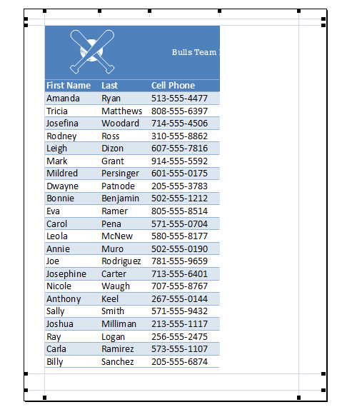
If some of your content is being cut off by the printer, you can use scaling to fit your workbook to the page automatically.- Navigate to the Print pane. In our example, we can see in the Preview pane that our content will be cut off when printed.
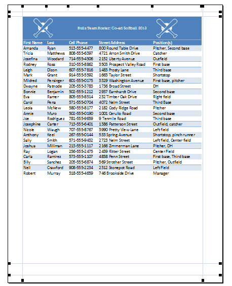
- Select the desired option from the Scaling drop-down menu. In our example, we'll select Fit Sheet on One Page.
Page Layout
Page Layout view
Before you start modifying a workbook's page layout, you may want to view the workbook in Page Layout view, which can help you visualize your changes.- To access Page Layout view, locate and select the Page Layout view command in the bottom-right corner of your workbook.

Page orientation
Excel offers two page orientation options: landscape and portrait. Landscape orients the page horizontally, while portrait orients the page vertically. Portrait is especially helpful for worksheets with a lot of rows, while landscape is best for worksheets with a lot of columns. In the example below, portrait orientation works best because the worksheet includes more rows than columns.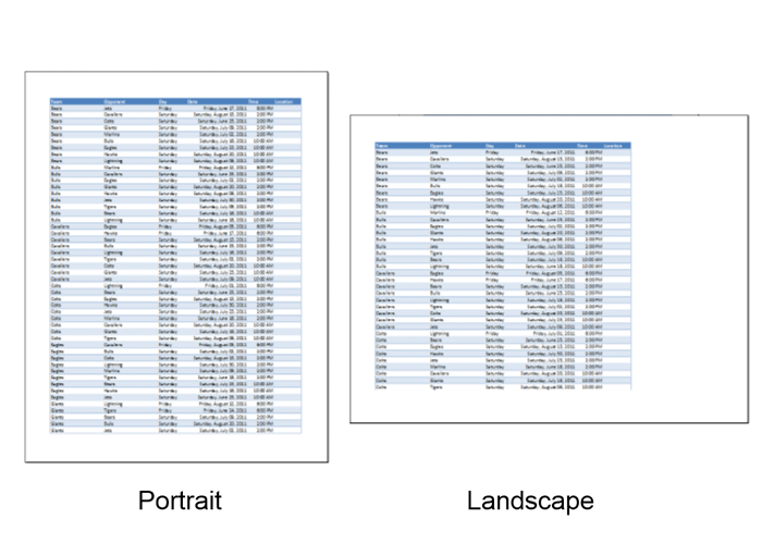
To change page orientation:

Slicers
You can insert slicers in Excel to quickly and easily filter pivot tables. However, using the report filter gives the exact same result.
Below you can find a two-dimensional pivot table. Go back to Pivot Tables to learn how to create this pivot table.

To insert a slicer, execute the following steps.
1. Click any cell inside the pivot table.
2. On the Analyze tab, in the Filter group, click Insert Slicer.
Below you can find a two-dimensional pivot table. Go back to Pivot Tables to learn how to create this pivot table.
To insert a slicer, execute the following steps.
1. Click any cell inside the pivot table.
2. On the Analyze tab, in the Filter group, click Insert Slicer.
Pivot Chart
Insert Pivot Chart | Filter Pivot Chart | Change Pivot Chart Type
A pivot chart is the visual representation of a pivot table in Excel. Pivot charts and pivot tables are connected with each other.Below you can find a two-dimensional pivot table. Go back to Pivot Tables to learn how to create this pivot table.

Insert Pivot Chart
To insert a pivot chart, execute the following steps.1. Click any cell inside the pivot table.
2. On the Analyze tab, in the Tools group, click PivotChart.

The Insert Chart dialog box appears.
3. Click OK.
Below you can find the pivot chart. This pivot chart will amaze and impress your boss.
Frequency Distribution
Remember, our data set consists of 213 records and 6 fields. Order ID, Product, Category, Amount, Date and Country.

First, insert a pivot table. Next, drag the following fields to the different areas.
1. Amount field to the Rows area.
2. Amount field (or any other field) to the Values area.

3. Click any cell inside the Sum of Amount column.
4. Right click and click on Value Field Settings.
Multi-level Pivot Table
Multiple Row Fields | Multiple Value Fields | Multiple Report Filter Fields
It's perfectly ok to drag more than one field to an area in a pivot table. We will look at an example of multiple row fields, multiple value fields and multiple report filter fields.Remember, our data set consists of 213 records and 6 fields. Order ID, Product, Category, Amount, Date and Country.

Multiple Row Fields
First, insert a pivot table. Next, drag the following fields to the different areas.1. Category field and Country field to the Rows area.
2. Amount field to the Values area.
Group Pivot Table Items
Group Products | Group Dates
This example teaches you how to group pivot table items. Learn how to group products and how to group dates by months.Below you can find a pivot table. Go back to Pivot Tables to learn how to create this pivot table.

Group Products
The Product field contains 7 items. Apple, Banana, Beans, Broccoli, Carrots, Mango and Orange.To create two groups, execute the following steps.
1. In the pivot table, select Apple and Banana.
2. Right click and click on Group.
PIVOT TABLE
Pivot Tables
Insert a Pivot Table | Drag fields | Sort | Filter | Change Summary Calculation | Two-dimensional Pivot Table
Pivot tables are one of Excel's most powerful features. A pivot table allows you to extract the significance from a large, detailed data set.Our data set consists of 213 records and 6 fields. Order ID, Product, Category, Amount, Date and Country.

Insert a Pivot Table
To insert a pivot table, execute the following steps.1. Click any single cell inside the data set.
2. On the Insert tab, in the Tables group, click PivotTable.

The following dialog box appears. Excel automatically selects the data for you. The default location for a new pivot table is New Worksheet.
3. Click OK.
Guide to the Excel Ribbon – Insert Tab
| Tables | |

|
 Pivot Table
- Summarize data using a Pivot Table. Pivot Table makes it easy to
arrange and summarize complicated data and drill down on details. |
 Table
- Create a table to manage and analyze related data. Tables make it
easy to sort, filter, and format data within a sheet. You can also use
the keyboard shortcut
Ctrl + T
to create a table. |
|
|
Illustrations
|
|

|
 Picture
- Insert a picture from a file. |
 Clip Art
- Insert Clip Art into the document, including movies, sounds, or stock photography to illustrate a specific concept. |
|
 Shapes
- Insert ready-made shapes, such as rectangles and circles, arrows, lines, flow chart symbols, and callouts. |
|
 SmartArt
- Insert a Smart Art graphic to visually communicate information. Smart
Art graphics range from graphical lists and process diagrams to more
complex graphics, such as Venn diagrams and organization charts.
Caution
! Using the SmartArt version of a Venn diagram does not make use of
everything you may want to do with a Venn. For example, you can not type
in the overlap area where you normally place shared characteristics of
the things you are comparing. To make a true Venn you should use the
circle tool in
Shapes
. | |
Guide to the Excel Ribbon – Home Tab
The Home Tab

When you open a new Excel Workbook the Home Tab is selected in view by default, not only because this is the first tab in the list but also because many of the everyday commands that you use can be found there.
The Home Tab along with the rest of the Excel Ribbon is customisable, but as this is a guide for beginners everything will be viewed from the default position which you get from a new installation of Excel so unless you have started any customising you should see the same view as this guide.
Tip: Hover the mouse cursor over any Icon on the Ribbon and a pop-up box will display what that Icon is for.
Command Groups
The various commands on the Home Tab are grouped in order to make the Ribbon as user-friendly as possible, the groupings listed are as follows (from left to right on the Ribbon):
1. The Clipboard Command Group
Within this Command Group you have Icons for Cut, Copy, Paste and Format Painter and they come in very useful when working with data in an Excel Workbook:

When you open a new Excel Workbook the Home Tab is selected in view by default, not only because this is the first tab in the list but also because many of the everyday commands that you use can be found there.
The Home Tab along with the rest of the Excel Ribbon is customisable, but as this is a guide for beginners everything will be viewed from the default position which you get from a new installation of Excel so unless you have started any customising you should see the same view as this guide.
Tip: Hover the mouse cursor over any Icon on the Ribbon and a pop-up box will display what that Icon is for.
Command Groups
The various commands on the Home Tab are grouped in order to make the Ribbon as user-friendly as possible, the groupings listed are as follows (from left to right on the Ribbon):
- Clipboard
- Font
- Alignment
- Number
- Styles
- Cells
- Editing
1. The Clipboard Command Group
Within this Command Group you have Icons for Cut, Copy, Paste and Format Painter and they come in very useful when working with data in an Excel Workbook:
- Cut: This command cuts data in preparation to move it to another location in the Excel Workbook.
- Copy: This command copies data in preparation to copy it to another location in your Excel Workbook.
- Paste: When you have either Cut or Copied data then you use the Paste command to paste it to the new location.
- Format Painter: Not as intuitive as the others but this command will copy the format of a cell and allow you to quickly apply it to other cells in your Workbook. For example if you have a cell that is a certain font type and you want to apply that font type to other cells you would click on the cell to copy (making it active) and the click the Format Painter command. You then click on the cell(s) that you want to apply that format on and Excel takes care of the rest.
ABOUT
About
Suggest Edits
BUSINESS INFO
Started on September 14, 2016
CONTACT INFO
@SunshineSITM
sitmsunshine@gmail.com
MORE INFO
About
Sunshine Institute of Technology & Management (SITM)
categories
Education · Magazine
Suggest Edits
BUSINESS INFO
Started on September 14, 2016
CONTACT INFO
@SunshineSITM
sitmsunshine@gmail.com
MORE INFO
About
Sunshine Institute of Technology & Management (SITM)
categories
Education · Magazine


Subscribe to:
Posts (Atom)